In [ ]:
Copied!
# 基本配置
## 常用包
import torch

## 超参数配置,有时也写入特定的文件中
batch_size = 16
lr = 1e-4 # 学习率
max_epoch = 100 # 训练轮数

## 硬件配置
def get_device(k=2):
    """
    智能选择训练设备
    - 如果有多个GPU,使用最后 k 个
    - 如果只有一个GPU,使用这一个
    - 如果没有GPU,回退到CPU
    """
    if torch.cuda.is_available():
        gpu_count = torch.cuda.device_count()
        print(f"GPU数量: {gpu_count}")
        if gpu_count >= k:
            device_ids = list(range(gpu_count-k, gpu_count))
        else:
            device_ids = list(range(gpu_count))
        print(f"使用GPU: {device_ids}")
        return torch.device(f"cuda:{device_ids[-1]}"), device_ids
    else:
        # 回退到CPU
        print("使用CPU")
        return torch.device("cpu"), None

device, device_ids = get_device(2)
# 基本配置
## 常用包
import torch
## 超参数配置,有时也写入特定的文件中
batch_size = 16
lr = 1e-4 # 学习率
max_epoch = 100 # 训练轮数
## 硬件配置
def get_device(k=2):
"""
智能选择训练设备
- 如果有多个GPU,使用最后 k 个
- 如果只有一个GPU,使用这一个
- 如果没有GPU,回退到CPU
"""
if torch.cuda.is_available():
gpu_count = torch.cuda.device_count()
print(f"GPU数量: {gpu_count}")
if gpu_count >= k:
device_ids = list(range(gpu_count-k, gpu_count))
else:
device_ids = list(range(gpu_count))
print(f"使用GPU: {device_ids}")
return torch.device(f"cuda:{device_ids[-1]}"), device_ids
else:
# 回退到CPU
print("使用CPU")
return torch.device("cpu"), None
device, device_ids = get_device(2)
GPU数量: 4
使用GPU: [2, 3]
In [ ]:
Copied!
# 简单网络构建
import torch
from torch import nn

class MLP(nn.Module):
    """
    Multi Layer Perceptron
    """
    def __init__(self, input_dim=784, hidden_dim=256, output_dim=10, **kwargs):
        super(MLP, self).__init__(**kwargs) # 继承父类的必要初始化
        self.hidden = nn.Linear(input_dim, hidden_dim) # 全连接层
        self.act = nn.ReLU() # 激活层
        self.output = nn.Linear(hidden_dim, output_dim)

    def forward(self, x):
        """
        A classic forward function, as neuron
        """
        o = self.act(self.hidden(x))
        return self.output(o)

X = torch.rand(2, 784)
mlp = MLP(input_dim=784, hidden_dim=256, output_dim=10)
mlp, mlp(X)
# 简单网络构建
import torch
from torch import nn
class MLP(nn.Module):
"""
Multi Layer Perceptron
"""
def __init__(self, input_dim=784, hidden_dim=256, output_dim=10, **kwargs):
super(MLP, self).__init__(**kwargs) # 继承父类的必要初始化
self.hidden = nn.Linear(input_dim, hidden_dim) # 全连接层
self.act = nn.ReLU() # 激活层
self.output = nn.Linear(hidden_dim, output_dim)
def forward(self, x):
"""
A classic forward function, as neuron
"""
o = self.act(self.hidden(x))
return self.output(o)
X = torch.rand(2, 784)
mlp = MLP(input_dim=784, hidden_dim=256, output_dim=10)
mlp, mlp(X)
Out[ ]:
(MLP(
   (hidden): Linear(in_features=784, out_features=256, bias=True)
   (act): ReLU()
   (output): Linear(in_features=256, out_features=10, bias=True)
 ),
 tensor([[ 0.1118, -0.3855,  0.1292, -0.2485, -0.0325, -0.2005,  0.1299,  0.1267,
          -0.0694, -0.0125],
         [ 0.0306, -0.3838,  0.0204, -0.3329, -0.1560, -0.2801,  0.1681,  0.0725,
          -0.1102, -0.0663]], grad_fn=<AddmmBackward0>))
In [5]:
Copied!
# 自定义网络层
class MCL(nn.Module):
    """
    Mean Center Layer
    """
    def __init__(self, **kwargs):
        super(MCL, self).__init__(**kwargs)
    def forward(self, x):
        return x - x.mean()

X = torch.arange(5, dtype=torch.float)
mcl = MCL()
mcl, mcl(X)
# 自定义网络层
class MCL(nn.Module):
"""
Mean Center Layer
"""
def __init__(self, **kwargs):
super(MCL, self).__init__(**kwargs)
def forward(self, x):
return x - x.mean()
X = torch.arange(5, dtype=torch.float)
mcl = MCL()
mcl, mcl(X)
Out[5]:
(MCL(), tensor([-2., -1., 0., 1., 2.]))
In [ ]:
Copied!
# 二维卷积层(含可学习参数)
# 注意下面实际操作使用了 nn.Conv2d,而不是我们的这个最小实现
class MyConv2d(nn.Module):
    """
    A simple convolutional layer
    :param kernel_size: kernel size
    """
    def __init__(self, kernel_size):
        super(MyConv2d, self).__init__()
        # random generate initial parameters
        self.weight = nn.Parameter(torch.randn(kernel_size))
        self.bias = nn.Parameter(torch.randn(1))

    def forward(self, x):
        return self.corr2d(x, self.weight) + self.bias

    def corr2d(X, K):
        """
        :param X: original matrix
        :param K: correlation kernel
        """
        h, w = K.shape
        X, K = X.float(), K.float()
        Y = torch.zeros((X.shape[0] - h + 1, X.shape[1] - w + 1))
        for i in range(Y.shape[0]):
            for j in range(Y.shape[1]):
                Y[i, j] = (X[i: i + h, j: j + w] * K).sum()
        return Y

# 定义一个函数来计算卷积层。它对输入和输出做相应的升维和降维
def comp_conv2d(conv2d, X):
    X = X.view((1, 1) + X.shape) # (1, 1)代表批量大小和通道数
    Y = conv2d(X)
    return Y.view(Y.shape[2:]) # 排除不关心的前两维:批量和通道

X = torch.rand(8, 8)
# 注意这里是两侧分别填充1⾏或列,所以在两侧一共填充2⾏或列
conv2d = nn.Conv2d(in_channels=1, out_channels=1, kernel_size=3,padding=1)
print(comp_conv2d(conv2d, X).shape)
# 当卷积核的高和宽不一致时填充也可以改变
conv2d = nn.Conv2d(in_channels=1, out_channels=1, kernel_size=(5, 3), padding=(2, 1))
print(comp_conv2d(conv2d, X).shape)
# 利用 stride 改变每次采样时滑动的步长
conv2d = nn.Conv2d(1, 1, kernel_size=(3, 5), padding=(0, 1), stride=(3, 4))
print(comp_conv2d(conv2d, X).shape)
# 二维卷积层(含可学习参数)
# 注意下面实际操作使用了 nn.Conv2d,而不是我们的这个最小实现
class MyConv2d(nn.Module):
"""
A simple convolutional layer
:param kernel_size: kernel size
"""
def __init__(self, kernel_size):
super(MyConv2d, self).__init__()
# random generate initial parameters
self.weight = nn.Parameter(torch.randn(kernel_size))
self.bias = nn.Parameter(torch.randn(1))
def forward(self, x):
return self.corr2d(x, self.weight) + self.bias
def corr2d(X, K):
"""
:param X: original matrix
:param K: correlation kernel
"""
h, w = K.shape
X, K = X.float(), K.float()
Y = torch.zeros((X.shape[0] - h + 1, X.shape[1] - w + 1))
for i in range(Y.shape[0]):
for j in range(Y.shape[1]):
Y[i, j] = (X[i: i + h, j: j + w] * K).sum()
return Y
# 定义一个函数来计算卷积层。它对输入和输出做相应的升维和降维
def comp_conv2d(conv2d, X):
X = X.view((1, 1) + X.shape) # (1, 1)代表批量大小和通道数
Y = conv2d(X)
return Y.view(Y.shape[2:]) # 排除不关心的前两维:批量和通道
X = torch.rand(8, 8)
# 注意这里是两侧分别填充1⾏或列,所以在两侧一共填充2⾏或列
conv2d = nn.Conv2d(in_channels=1, out_channels=1, kernel_size=3,padding=1)
print(comp_conv2d(conv2d, X).shape)
# 当卷积核的高和宽不一致时填充也可以改变
conv2d = nn.Conv2d(in_channels=1, out_channels=1, kernel_size=(5, 3), padding=(2, 1))
print(comp_conv2d(conv2d, X).shape)
# 利用 stride 改变每次采样时滑动的步长
conv2d = nn.Conv2d(1, 1, kernel_size=(3, 5), padding=(0, 1), stride=(3, 4))
print(comp_conv2d(conv2d, X).shape)
Conv2d(1, 1, kernel_size=(3, 3), stride=(1, 1), padding=(1, 1))
Out[ ]:
torch.Size([8, 8])
In [ ]:
Copied!
# 池化层
# 池化层可以看作是卷积核特殊的卷积层,但是进行的操作一般是顺序无关的操作
class MyPool2d(nn.Module):
    """
    simple pooling layer
    """
    def __init__(self, pool_size, mode="mean"):
        super(MyPool2d, self).__init__()
        self.pool_size = pool_size
        self.mode = mode

    def forward(self, x):
        return self.pool2d(x, self.pool_size, mode=self.mode)

    def pool2d(self, X, pool_size, mode="mean"):
        p_h, p_w = pool_size
        Y = torch.zeros((X.shape[0] - p_h + 1, X.shape[1] - p_w + 1))
        for i in range(Y.shape[0]):
            for j in range(Y.shape[1]):
                if mode == 'mean':
                    Y[i, j] = X[i: i + p_h, j: j + p_w].mean()
                elif mode == 'max':
                    Y[i, j] = X[i: i + p_h, j: j + p_w].max()
        return Y

X = torch.tensor([[0, 1, 2], [3, 4, 5], [6, 7, 8]], dtype=torch.float)
mypool2d = MyPool2d(pool_size=(2, 2))
mypool2d, mypool2d(X)
# 池化层
# 池化层可以看作是卷积核特殊的卷积层,但是进行的操作一般是顺序无关的操作
class MyPool2d(nn.Module):
"""
simple pooling layer
"""
def __init__(self, pool_size, mode="mean"):
super(MyPool2d, self).__init__()
self.pool_size = pool_size
self.mode = mode
def forward(self, x):
return self.pool2d(x, self.pool_size, mode=self.mode)
def pool2d(self, X, pool_size, mode="mean"):
p_h, p_w = pool_size
Y = torch.zeros((X.shape[0] - p_h + 1, X.shape[1] - p_w + 1))
for i in range(Y.shape[0]):
for j in range(Y.shape[1]):
if mode == 'mean':
Y[i, j] = X[i: i + p_h, j: j + p_w].mean()
elif mode == 'max':
Y[i, j] = X[i: i + p_h, j: j + p_w].max()
return Y
X = torch.tensor([[0, 1, 2], [3, 4, 5], [6, 7, 8]], dtype=torch.float)
mypool2d = MyPool2d(pool_size=(2, 2))
mypool2d, mypool2d(X)
Out[ ]:
(MyPool2d(),
 tensor([[2., 3.],
         [5., 6.]]))
In [ ]:
Copied!
# 模型初始化
# 在 https://pytorch.org/docs/stable/nn.init.html 可以看到模型初始化的一些方法;以 `_` 结尾表明这些方法对 tensor 本身进行操作,会自动选择合适的方法进行初始化;当然要主动选择初始化方式也没有问题。
conv = nn.Conv2d(1, 3, 3)
linear = nn.Linear(10, 1)
conv.weight.data # 默认
# 模型初始化
# 在 https://pytorch.org/docs/stable/nn.init.html 可以看到模型初始化的一些方法;以 `_` 结尾表明这些方法对 tensor 本身进行操作,会自动选择合适的方法进行初始化;当然要主动选择初始化方式也没有问题。
conv = nn.Conv2d(1, 3, 3)
linear = nn.Linear(10, 1)
conv.weight.data # 默认
Out[ ]:
tensor([[[[ 0.1596,  0.1404,  0.1189],
          [-0.2656, -0.0942, -0.2529],
          [-0.0582, -0.1957,  0.1201]]],


        [[[-0.2217,  0.1839, -0.1353],
          [ 0.0787, -0.0343,  0.2490],
          [ 0.1572,  0.2899,  0.1347]]],


        [[[-0.0085, -0.1805, -0.3324],
          [ 0.2490,  0.1714,  0.2518],
          [ 0.2316,  0.0324,  0.2219]]]])
定义模型 
层 
基于 nn.Module,我们可以通过 Sequential,ModuleList 和 ModuleDict 三种方式定义 PyTorch 模型。他们在 nn/modules/container.py 中被定义。
Sequential
顾名思义,当模型的前向计算只是简单的串联时,Sequential 是一个比较简单的模型定义方式。它可以接收一个子模块的有序字典 (OrderedDict) 或者一系列子模块作为参数来逐一添加 Module 的实例。最大的优势是简单。
from collections import OrderedDict
class Sequential(nn.Module):
    _modules: dict[str, Module]  # type: ignore[assignment]
    def __init__(self, *args):
        super(Sequential, self).__init__()
        if len(args) == 1 and isinstance(args[0], OrderedDict): # 如果传入的是一个OrderedDict
            for key, module in args[0].items():
                self.add_module(key, module)  # add_module方法会将module添加进self._modules
        else:  # 传入的是一些Module
            for idx, module in enumerate(args):
                self.add_module(str(idx), module)
    def forward(self, input):
        # self._modules返回一个 OrderedDict,保证会按照成员添加时的顺序遍历成
        for module in self._modules.values():
            input = module(input)
        return input
In [ ]:
Copied!
# sequential
net1 = nn.Sequential(
        nn.Linear(784, 256),
        nn.ReLU(),
        nn.Linear(256, 10))
print(net1)

from collections import OrderedDict
net2 = nn.Sequential(OrderedDict([
          ('fc1', nn.Linear(784, 256)),
          ('relu1', nn.ReLU()),
          ('fc2', nn.Linear(256, 10))
          ]))
print(net2)
# sequential
net1 = nn.Sequential(
nn.Linear(784, 256),
nn.ReLU(),
nn.Linear(256, 10))
print(net1)
from collections import OrderedDict
net2 = nn.Sequential(OrderedDict([
('fc1', nn.Linear(784, 256)),
('relu1', nn.ReLU()),
('fc2', nn.Linear(256, 10))
]))
print(net2)
ModuleList
ModuleList 接收一个子模块(或层,需属于 nn.Module 类)的列表作为输入,然后也可以类似 List 那样进行 append 和 extend 操作。同时,子模块或层的权重也会自动添加到网络中来。
要特别注意的是,nn.ModuleList 并没有定义一个网络,它只是将不同的模块储存在一起。ModuleList 中元素的先后顺序并不代表其在网络中的真实位置顺序,需要经过 forward 函数指定各个层的先后顺序后才算完成了模型的定义。
class ModuleList(Module):
    _modules: dict[str, Module]  # type: ignore[assignment]

    def __init__(self, modules: Optional[Iterable[Module]] = None) -> None:
        super().__init__()
        if modules is not None:
            self += modules

    # remove forward altogether to fallback on Module's _forward_unimplemented
In [ ]:
Copied!
# ModuleList
net3 = nn.ModuleList([nn.Linear(784, 256), nn.ReLU()])
net3.append(nn.Linear(256, 10)) # # 类似List的append操作
print(net3[-1])  # 类似List的索引访问
print(net3)
# ModuleList
net3 = nn.ModuleList([nn.Linear(784, 256), nn.ReLU()])
net3.append(nn.Linear(256, 10)) # # 类似List的append操作
print(net3[-1]) # 类似List的索引访问
print(net3)
ModuleDict
ModuleDict 和 ModuleList 的作用类似,只是 ModuleDict 能够更方便地为神经网络的层添加名称。
In [ ]:
Copied!
# ModuleDict
net3 = nn.ModuleDict({
    'linear': nn.Linear(784, 256),
    'act': nn.ReLU(),
})
net3['output'] = nn.Linear(256, 10) # 添加
print(net3['linear']) # 访问
print(net3.output)
print(net3)
# ModuleDict
net3 = nn.ModuleDict({
'linear': nn.Linear(784, 256),
'act': nn.ReLU(),
})
net3['output'] = nn.Linear(256, 10) # 添加
print(net3['linear']) # 访问
print(net3.output)
print(net3)
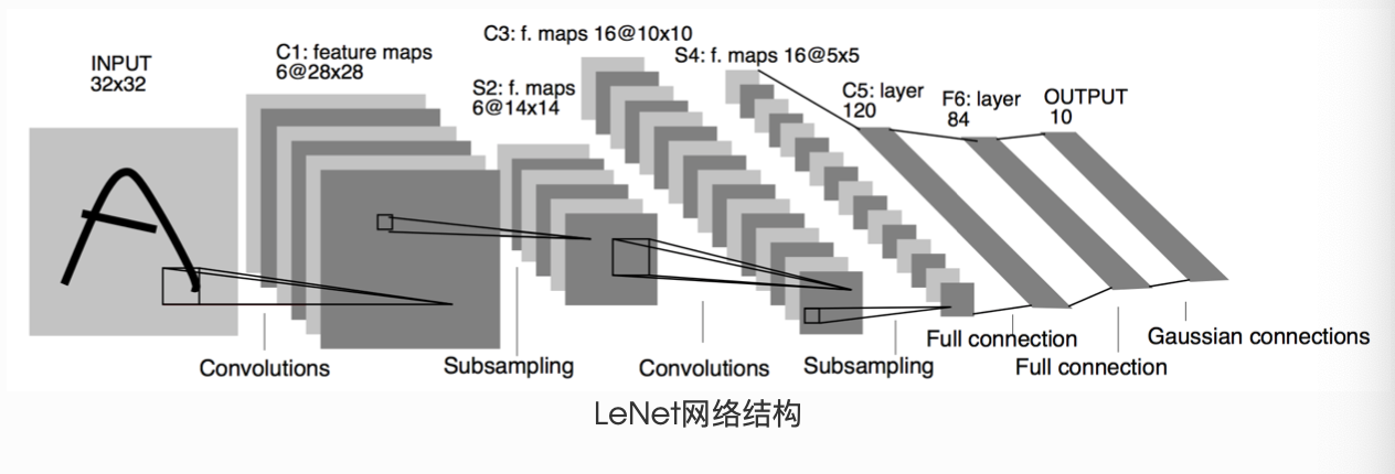
LeNet & AlexNet
LeNet 是一个简单的前馈神经网络 (feed-forward network)。它接受一个输入,然后将它送入下一层,一层接一层的传递,最后给出输出。
一个神经网络的典型训练过程如下:
- 定义包含一些可学习参数(或者叫权重)的神经网络
- 在输入数据集上迭代
- 通过网络处理输入
- 计算 loss(输出和正确答案的距离)
- 将梯度反向传播给网络的参数
- 更新网络的权重,一般使用一个简单的规则:weight = weight - learning_rate * gradient
In [ ]:
Copied!
# LeNet
import torch.nn.functional as F

class LeNet(nn.Module):

    def __init__(self):
        super(LeNet, self).__init__()
        # 输入图像channel:1;输出channel:6;5x5卷积核
        self.conv1 = nn.Conv2d(1, 6, 5)
        self.conv2 = nn.Conv2d(6, 16, 5)
        # an affine operation: y = Wx + b
        self.fc1 = nn.Linear(16 * 5 * 5, 120)
        self.fc2 = nn.Linear(120, 84)
        self.fc3 = nn.Linear(84, 10)

    def forward(self, x):
        # 2x2 Max pooling
        x = F.max_pool2d(F.relu(self.conv1(x)), (2, 2))
        # 如果是方阵,则可以只使用一个数字进行定义
        x = F.max_pool2d(F.relu(self.conv2(x)), 2)
        x = x.view(-1, self.num_flat_features(x))
        x = F.relu(self.fc1(x))
        x = F.relu(self.fc2(x))
        x = self.fc3(x)
        return x

    def num_flat_features(self, x):
        size = x.size()[1:]  # 除去批处理维度的其他所有维度
        num_features = 1
        for s in size:
            num_features *= s
        return num_features

lenet = LeNet()
params = list(lenet.parameters())
# Net 自动将 Conv2d 和 Linear 的权重和偏置注入到模型中,5层网络,len(params)=10
len(params), params[0].size(), params[1].size()
# (10, torch.Size([6, 1, 5, 5]), torch.Size([6]))
output = lenet(torch.randn(1, 1, 32, 32))
lenet.zero_grad()
output.backward(torch.randn(1, 10))
# LeNet
import torch.nn.functional as F
class LeNet(nn.Module):
def __init__(self):
super(LeNet, self).__init__()
# 输入图像channel:1;输出channel:6;5x5卷积核
self.conv1 = nn.Conv2d(1, 6, 5)
self.conv2 = nn.Conv2d(6, 16, 5)
# an affine operation: y = Wx + b
self.fc1 = nn.Linear(16 * 5 * 5, 120)
self.fc2 = nn.Linear(120, 84)
self.fc3 = nn.Linear(84, 10)
def forward(self, x):
# 2x2 Max pooling
x = F.max_pool2d(F.relu(self.conv1(x)), (2, 2))
# 如果是方阵,则可以只使用一个数字进行定义
x = F.max_pool2d(F.relu(self.conv2(x)), 2)
x = x.view(-1, self.num_flat_features(x))
x = F.relu(self.fc1(x))
x = F.relu(self.fc2(x))
x = self.fc3(x)
return x
def num_flat_features(self, x):
size = x.size()[1:] # 除去批处理维度的其他所有维度
num_features = 1
for s in size:
num_features *= s
return num_features
lenet = LeNet()
params = list(lenet.parameters())
# Net 自动将 Conv2d 和 Linear 的权重和偏置注入到模型中,5层网络,len(params)=10
len(params), params[0].size(), params[1].size()
# (10, torch.Size([6, 1, 5, 5]), torch.Size([6]))
output = lenet(torch.randn(1, 1, 32, 32))
lenet.zero_grad()
output.backward(torch.randn(1, 10))
Out[ ]:
tensor([[ 0.1366, -0.0211, -0.0219, -0.2076, -0.1440, -0.0762,  0.0472, -0.0896,
          0.1511, -0.0552]], grad_fn=<AddmmBackward0>)
In [ ]:
Copied!
# AlexNet
class AlexNet(nn.Module):
    """
    AlexNet https://datawhalechina.github.io/thorough-pytorch/_images/3.4.2.png
    """
    def __init__(self):
        super(AlexNet, self).__init__()
        self.conv = nn.Sequential(
            nn.Conv2d(1, 96, kernel_size=11, stride=4), # in_channels, out_channels, kernel_size, stride, padding
            nn.ReLU(),
            nn.MaxPool2d(3, 2), # kernel_size, stride
            # 减小卷积窗口,使用填充为2来使得输入与输出的高和宽一致,且增大输出通道数
            nn.Conv2d(96, 256, 5, 1, 2),
            nn.ReLU(),
            nn.MaxPool2d(3, 2),
            # 连续3个卷积层,且使用更小的卷积窗口。除了最后的卷积层外,进一步增大了输出通道数。
            # 前两个卷积层后不使用池化层来减小输入的高和宽
            nn.Conv2d(256, 384, 3, 1, 1),
            nn.ReLU(),
            nn.Conv2d(384, 384, 3, 1, 1),
            nn.ReLU(),
            nn.Conv2d(384, 256, 3, 1, 1),
            nn.ReLU(),
            nn.MaxPool2d(3, 2)
        )
         # 这里全连接层的输出个数比LeNet中的大数倍。使用 Dropout 层来缓解过拟合
        self.fc = nn.Sequential(
            nn.Linear(256*5*5, 4096),
            nn.ReLU(),
            nn.Dropout(0.5),
            nn.Linear(4096, 4096),
            nn.ReLU(),
            nn.Dropout(0.5),
            # 输出层。由于这里使用Fashion-MNIST,所以用类别数为10,而非论文中的1000
            nn.Linear(4096, 10),
        )

    def forward(self, img):
        feature = self.conv(img)
        output = self.fc(feature.view(img.shape[0], -1))
        return output
# AlexNet
class AlexNet(nn.Module):
"""
AlexNet https://datawhalechina.github.io/thorough-pytorch/_images/3.4.2.png
"""
def __init__(self):
super(AlexNet, self).__init__()
self.conv = nn.Sequential(
nn.Conv2d(1, 96, kernel_size=11, stride=4), # in_channels, out_channels, kernel_size, stride, padding
nn.ReLU(),
nn.MaxPool2d(3, 2), # kernel_size, stride
# 减小卷积窗口,使用填充为2来使得输入与输出的高和宽一致,且增大输出通道数
nn.Conv2d(96, 256, 5, 1, 2),
nn.ReLU(),
nn.MaxPool2d(3, 2),
# 连续3个卷积层,且使用更小的卷积窗口。除了最后的卷积层外,进一步增大了输出通道数。
# 前两个卷积层后不使用池化层来减小输入的高和宽
nn.Conv2d(256, 384, 3, 1, 1),
nn.ReLU(),
nn.Conv2d(384, 384, 3, 1, 1),
nn.ReLU(),
nn.Conv2d(384, 256, 3, 1, 1),
nn.ReLU(),
nn.MaxPool2d(3, 2)
)
# 这里全连接层的输出个数比LeNet中的大数倍。使用 Dropout 层来缓解过拟合
self.fc = nn.Sequential(
nn.Linear(256*5*5, 4096),
nn.ReLU(),
nn.Dropout(0.5),
nn.Linear(4096, 4096),
nn.ReLU(),
nn.Dropout(0.5),
# 输出层。由于这里使用Fashion-MNIST,所以用类别数为10,而非论文中的1000
nn.Linear(4096, 10),
)
def forward(self, img):
feature = self.conv(img)
output = self.fc(feature.view(img.shape[0], -1))
return output